The goal of the Connectivity Map (CMap) is to build a resource of gene expression profiles to aid biomedical research and therapeutic discovery. The core CMap technology is an assay called L1000, which measures gene expression changes in cells. L1000 achieves a significant increase in throughput and a significant decrease in cost as compared to other gene expression technologies due in large part to the practice of measuring two genes using the same physical material (in this case, microscopic beads). After data collection, the expression values of the two genes are computationally extracted in a process called "peak deconvolution". The current implementation, an algorithm called D-Peak, is effective but imperfect, and hence the aim of this contest is to improve D-Peak, which we hypothesize will enable CMap to produce higher quality data more efficiently.

If you want to learn the science behind CMap and L1000, see the Background section in the very bottom of this page, and/or visit the CMap website at clue.io.

This match is rated and TCO-eligible. Threshold for TCO-eligibility: 10% improvement of the benchmark solution score on the final test dataset.

Registration / submission deadline: 09:00 AM ET on January 18, 2019

The Problem

For the purpose of this challenge, the core CMap technology can be described as follows.

In a single experiment, CMap makes 488 measurements. Each measurement produces an intensity histogram (a list of integers), which characterizes expression of two distinct genes in the sample (for a total of 488 x 2 = 976 genes). In the ideal case, each histogram consists of two peaks (see Figure 1), each corresponding to a single gene. The genes are mixed in 2:1 ratio, thus the areas under the peaks have 2:1 ratio, which allows us to associate each peak with the specific gene. The median position of each peak corresponds to the gene's expression level, and that's what you need to determine in this challenge.

For training purposes, you are given two sets of about 384 experiments each (a total of 488 x 384 = 187,392  measurements, with each histogram consisting of ~50 - 100 observations); and you are asked to develop code that takes each set as input, deconvolutes the data, and returns a matrix with the median position of each peak for the 976 genes (rows) in the approximately 384 experiments (columns). 

The resulting deconvoluted (DECONV) data will be compared against the corresponding data obtained by a more accurate, yet more expensive, measurement strategy, called "UNI", in which each measurement is focused on a single gene (see the Scoring section below).

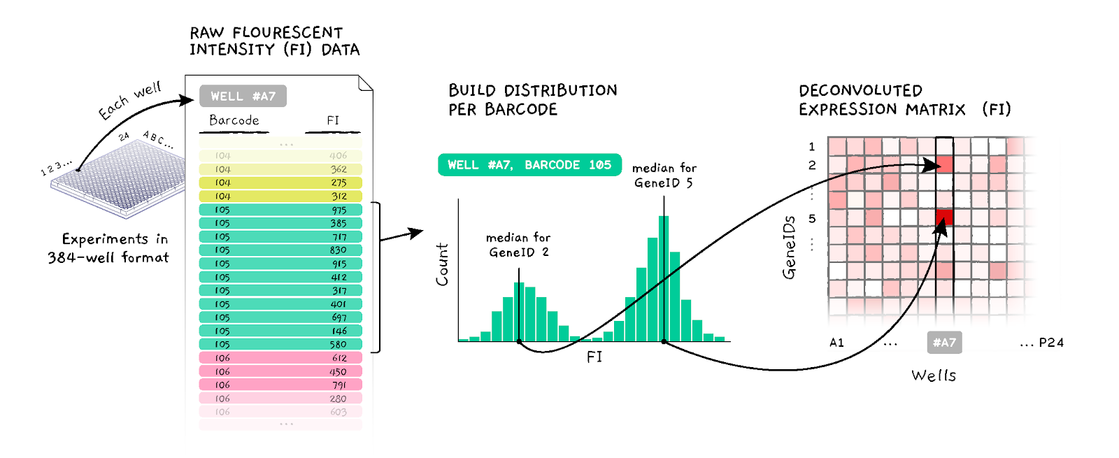
Figure 1. D-Peak algorithm schematics

Current Benchmark Solution. CMap's current solution to this problem is based on a K-means clustering algorithm that works as follows. For each measurement, the K-means clustering algorithm partitions the list of realizations into K >= 2 distinct clusters and identifies two of the clusters whose ratio of membership is as close as possible to 2:1. The algorithm, then, takes the median for each of the two clusters, assigning these values to the appropriate gene (i.e., matching clusters with more observations to the gene mixed in higher proportion).

Known problems with the current approach are that the K-means algorithm is generally a biased and inconsistent estimator of the peaks of a bimodal distribution and, it fails sometimes to detect peaks with few observations, or it incorrectly identifies these peaks as 3^rd peaks, disregarding them. Another limitation is that the K-means clustering algorithm is computationally costly and, hence, expensive for data generation at scale (current Matlab implementation, with some additional post-processing, takes about 30 minutes on a 12-core server to process sets of 384 experiments).

Input Data

Each of training, provisional, and final datasets consits of two sets of experiments. A single set of experiments is represented by a folder containing ~384 tab-separated files, one per experiment. The folder is named after the set, e.g. DPK.CP001_A549_24H_X1_B42, and each file in that folder is named appending a 3-symbol experiment label and file extension, like _B14.txt, resulting in the names like DPK.CP001_A549_24H_X1_B42_B14.txt (these names encode additional information that is irrelevant to you).

Each of these files has two columns: one identifying the measurement (barcode_id) and one with the realizations (FI). Measurements have approximately the same number of realizations, although there is variability due to detection failure.

An additional file (barcode_to_gene_map.txt) contains a mapping between each unique measurement (barcode_id) and the two genes (gene_id) it measures in DUO mode; it also includes a column (high_prop) that indicates which gene of the pair is mixed in higher (=1) or lower (=0) proportion.

Output Data

For each input dataset your code will generate a matrix of non-negative numbers, representing estimated median intensities, for 976 genes (rows) in approximately 384 experiments (columns).

The matrix will be written out into a GCT file, named the same way as the folder containing the test set, with .gct file extension appended in the end. The GCT format is a tab-delimetered text file that describes an expression dataset (see here). Example GCT files will be provided in the competitor pack.

Submission Format

You will submit a dockerized version of your algorithm. The scoring system will build a Docker container out of it, and will run it for each of test sets, passing in four arguments: --dspath PATH/TO/INPUT/DATASET/FOLDER, --out /PATH/TO/OUTPUT/FOLDER, --create_subdir 0, and --plate TEST_SET_NAME. The first argument points to the folder containing ~384 experiment files; the second argument point to the folder where you will write the output GCT file; the third argument to be ignored, it is there just for compatibility with the benchmark solution; and the last argument tells you how to name the output file.

In the challenge forum you will find competitor pack with local test & score harness, and basic instructions for dockerization of your algorithms. In case of any Docker-related problems, do not hesitate to ask help in the forum.

The online scoring system and leaderboard will become available a few days after the match launch.

Scoring

Your submissions will be scored based on accuracy and speed.

Regarding accuracy, we will compare your outcomes with the corresponding data obtained by a more accurate, yet more expensive, gene expression technology, called ‘UNI’, in which each bead type is used to measure a single gene. 

The scoring function combines two measures of accuracy: one component of which is applied to deconvoluted (DECONV) data and one to differential expression (DE) data. DE is derived from DECONV by applying a series of transformations (parametric scaling, quantile normalization, and robust z-scoring) that are described in detail below and in Subramanian et al. 2017. The local test & score harness performs DECONV > DE transformation as a part of the scoring, and keeps intermediate results, in case you need DE data.

The reason for scoring DE data is because it is at this level where the most interesting gene expression changes are observed. Of particular interest is obtaining significant improvement in the detection of, so called, “extreme modulations.” These are genes that, after a series of necessary transformations, exhibit an exceedingly high (or low) DE values relative to a fixed threshold. It is therefore desirable to assess accuracy here as well as DECONV.

The specific accuracy metrics are described below and outlined in Figure 2.


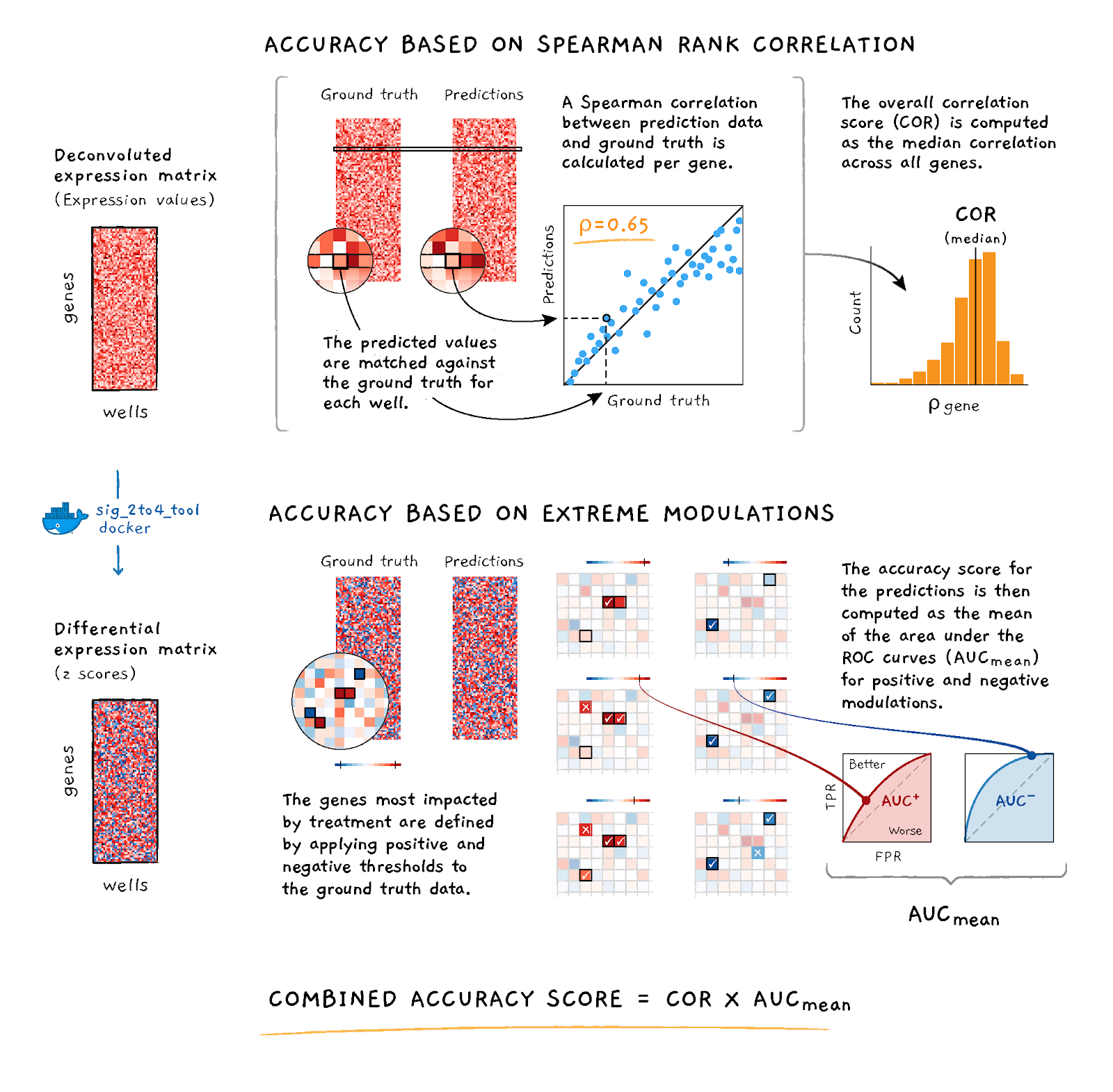
Figure 2. Accuracy scoring schematic

Accuracy Based on Spearman Correlation

The first component of the scoring function is based on the Spearman rank correlation between the provided DECONV data and the corresponding UNI data.

For a given dataset p, let M_{DUO, p} and M_{UNI, p} denote the matrices of the estimated gene intensities for G = 976 genes (rows) and S ~ 384 experiments (columns) under DUO and UNI detection.  Compute the Spearman rank correlation matrix between the rows of M_{DUO, p} and the rows of M_{UNI, p}; take the median of the diagonal elements of the resulting matrix (i.e., the values corresponding to the matched experiments between UNI and DUO) to compute the median correlation per dataset:

COR_p = median(diag(spearman(M_{DUO, p}, M_{UNI, p}))

Accuracy Based on AUC

The second component of the scoring function is based on the Area Under the receiver operating characteristic Curve (AUC) that uses the competitor's DE values at various thresholds to predict the UNI's DE values being higher than 2 ("high") or lower than -2 ("low").
 
For a given bead type a in a given dataset p, let AUC_{p, c} denote the corresponding area under the curve where c = { high | low }, where high means UNI_{DE, p} >= 2, and low means UNI_{DE, p} <= −2; then, compute the arithmetic mean of the area under the curve per class to obtain the corresponding score per dataset:

AUC_p = (AUC_{p, hight} + AUC_{p, low}) / 2

Speed Component of the Score

For a given dataset p, the time component of the score is computed as the run time in seconds for deconvoluting the data in both test cases: Runtime_p

Notice that multi-theading is allowed in this match, and thus highly recommended. Your submission will be tested on multi-core machines (presumably, 8 cores). The maximum execution time of your solution will be capped by 30 minutes.

Aggregated Score

SCORE = MAX_SCORE * (MAX(COR_p, 0))² * AUC_p² * exp(- T_solution / (3 * T_benchmark) )
where T_benchmark is the deconvolution time required by the reference DPeak implementation
 

Elibility Criteria

To be eligible for prizes, in addition to the standard Topcoder eligibility criteria, you'll have to:

• Get a prize-eligible position in the final testing after the match (be in Top-9 scores), with a score above the threshold, which will be declared once the online scoring system is up (the threshold score will express a 10% rise in accuracy and performance over the benchmark Matlab implementation of DPeak algorithm);
• Provide a full source code of your solution, and any related assets;
• Within 7 days after the announcement of final results, provide a write-up on your algorithm;

Appendix

Description of Connectivity Map and L1000

The Connectivity Map (CMap) project at the Broad Institute utilizes a novel gene expression profiling technology to generate gene expression profiles at scale. This new technology uses an assay called L1000 to measure gene expression of a select subset of approximately 1,000 genes, called landmarks. This procedure enables researchers to study the connections between genes, drugs, and diseases at a large scale (Subramanian et al. 2017).

The core CMap experiment is to treat cultured cells with various perturbations and measure the corresponding gene expression response using L1000. The L1000 assay is based on Luminex bead technology and uses multiple bead types to simultaneously measure the expression of many genes. When the beads are scanned, two values are obtained from each bead: one indicating the color of the bead (the target analyte) and the other indicating the intensity of the signal, which is a reflection of mRNA expression (Appendix Figure 1 below). The beads are read on a dual-laser flow-based scanner. One laser classifies the bead and determines the bead type that is being detected. The second laser determines the magnitude of the PE-derived signal, which is in direct proportion to the amount of bound analyte.


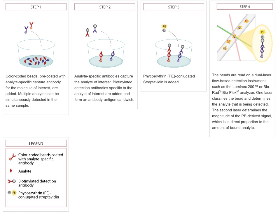
Appendix Figure 1. Luminex detection schematic. Reproduced from https://www.rndsystems.com/resources/technical/luminex-bead-based-assay-principle. In the CMap application, oligonucleotides are used instead of antibodies, but the overall principle remains the same.

Although the scanner is designed to detect only 500 different bead types, CMap uses it to measure ~1000 landmark genes (978 genes to be exact). Of the 500 available types, 12 are used to measure controls. The remaining 488 colors are each used to measure two genes. The 976 landmark genes (excluding two genes that are measured independently) are grouped into pairs and coupled to beads of the same color. Genes coupled to the same bead color are combined in a ratio of 2:1 prior to use. So, the detected signal intensity for each bead color provides a composite measure of the abundance of the transcripts of the two genes.

The main problem is to split this composite measure into two individual intensity values, one for each of the genes coupled with the same bead color.
To deconvolute the composite expression signal into two values and associate them with the appropriate genes, CMap employs an algorithm called "dpeak". The basic elements of the algorithm are as follows, but more details can be found at https://clue.io/connectopedia/measuring_expr_of_1000_genes.

• It constructs a histogram of fluorescence intensity values for all beads of a specific color. This yields a distribution that generally consists of two peaks (as in the Figure below): a larger one that designates expression of the gene for which a larger proportion of beads are present, and a smaller peak representing the other gene. 
• Using a k-means clustering algorithm, the distribution is partitioned into two distinct clusters, such that the ratio of cluster membership is as close as possible to 2:1, and the median expression value for each cluster is then assigned as the expression value of the appropriate gene. 
• In cases where two peaks are not resolvable, the median expression of the distribution is assigned to both genes. 

The current implementation also carries out plate-level adjustments after running dpeak on all samples from the same plate.

Known issues / challenges to overcome:

• Sometimes the algorithm fails to detect peaks with low memberships or incorrectly identify them as 3rd peaks
• The k-means clustering is generally biased and inconsistent estimator of the gene distributions (Jin 2016)
• Errors are more frequent when few (less than ~30) beads are observed

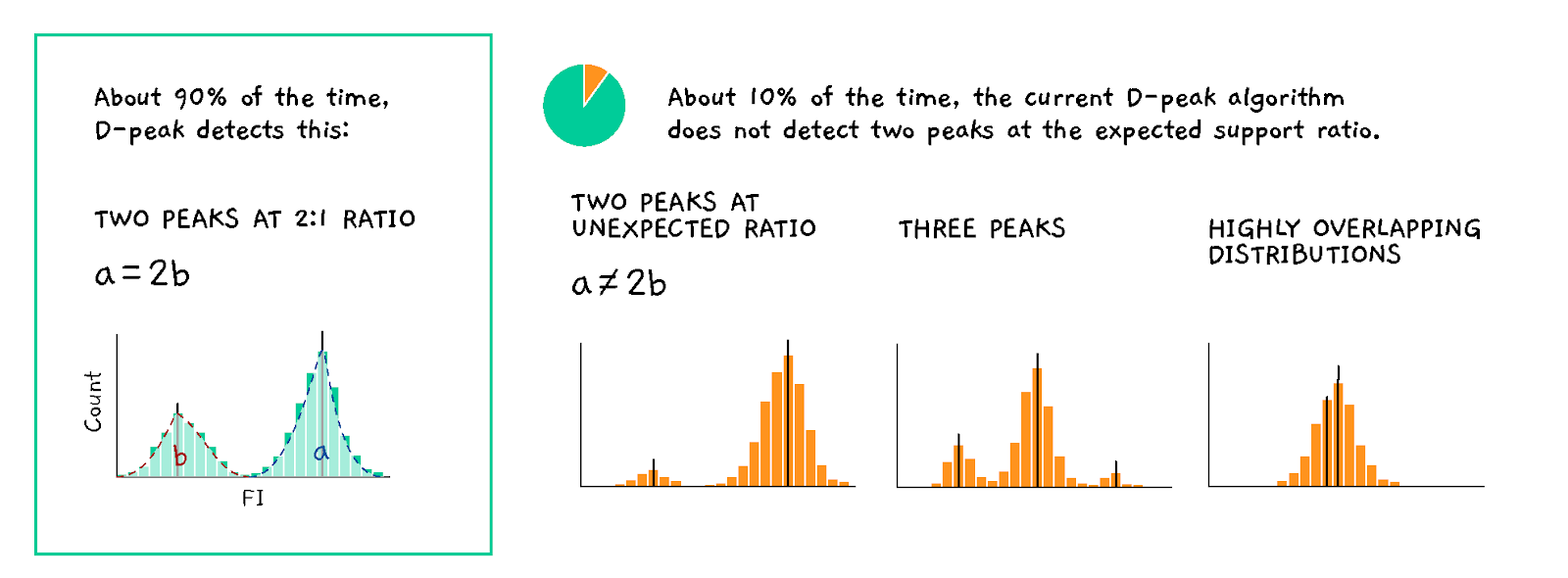
Appendix Figure 2. D-Peak error modes.

Additional adjustments made by CMap k-means implementation

The current implementation also applies a heuristic, called flip-adjust, which aims to identify and correct instances where the two peaks may have been misassigned. After dpeak has run, flip-adjust collects all data across all wells in the given plate for a given analyte. It then performs a two-class linear discriminant analysis (LDA) on the plate-wide data using both the bead count and deconvoluted expression values as features (Appendix Figure 3 below). It then uses the discriminator to try and classify the count/expression data from every sample in every well. If the two genes from the same well are simultaneously misclassified, according to the dpeak-assigned labels, then these labels are reversed. This is based on the assumption that it is highly improbable that both genes on the same analyte in the same well will have count and expression values that deviate widely from the plate-wide population. Empirically we observe that flip-adjust only impacts a very small percentage of all data, but competitors may find useful the concept of leveraging data across multiple wells.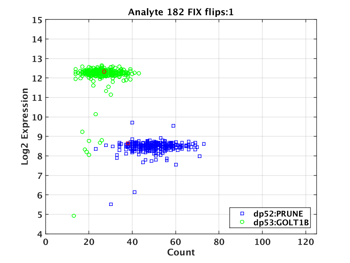


Appendix Figure 3. Example of a flip adjustment. A scatter plot of the log2 deconvoluted expression vs. the bead count for the two genes assigned to a given bead type in a given plate. The points highlighted in red are those where the deconvoluted value for the dp52 gene is predicted to be in the dp53 population and vice versa, and hence the gene assignments were reversed.

GCT Format

GCT (Gene Cluster Text) is a tab-delimited text file format for storing matrix data. Each column represents a specific experiment (e.g. treatment with a small-molecule drug) and each row represents genes that are measured in the L1000 assay. In this contest, GCT matrix dimensions are encoded into the filename. For example, the file DPK.CP001_A549_24H_X1_B42_n376x976.gct contains 376 columns and 976 rows. For more information on the GCT format, please see https://clue.io/connectopedia/gct_format.

Data Transformation

Data are transformed from DECONV to DE using the steps outlined below, and in Subramanian et al. 2017.

1. Invariant set normalization
   
   We use a rescaling procedure called L1000 Invariant Set Scaling, or LISS, involving 80 control transcripts (8 each at 10 levels of low to high expression) that we empirically found to be invariant in historic, non-L1000 data. The 80 genes are used to construct a calibration curve for each sample. Each curve is computed using the median expression of the 8 invariant genes at each of the 10 pre-defined invariant levels. We then loess-smooth the data and fit the following power law function using non-linear least squares regression:
   
   y=ax^b+c
   
   where x is the unscaled data and a, b, and c are constants estimated empirically. The entire sample is then rescaled using the obtained model.
    
2. Quantile normalization
   
   We then standardize the shape of the expression profile distributions on each plate by applying quantile normalization, or QNORM. This is done by first sorting each profile by expression level, and then normalizing the data by setting the highest-ranking value in each profile to the median of all the highest ranking values, the next highest value to the median of the next highest values, and so on down to the data for the lowest expression level. 
    
3. Robust Z-scoring
   
   To obtain a measure of relative gene expression, we use a robust z-scoring procedure to generate differential expression values from normalized profiles. We compute the differential expression of gene x in the ith sample on the plate as:
   
   ( x_i - median(X) ) / ( 1.4826  MAD(X) )
   
   where X is the vector of normalized gene expression of gene x across all samples on the plate, MAD is the median absolute deviation of X, and the factor of 1.4826 is a scaling constant to rescale the data as if the standard deviation were used instead of the median absolute deviation.