May 4, 2017 TCO17 Marathon Round 1: An Analysis

The submission phase of TCO17 Marathon Round 1 ended on April, 26. Many competitors submitted quite good solutions since the middle of the match. 7 people: chokudai, wleite, blackmath, Psyho, atsT5515, tomerun and nhzp339 reached an impressive 790, 000+ provisional score. 8 more people reached 780, 000+ score, which is in my opinion also quite good for this task.

Leaders’ approach

There seem to be 2 competing metaheuristics to this task: Simulated Annealing (SA) and Spring-force based methods (SF). If you have not checked an article on the first one, hurry to read it here.
After analyzing the top solutions, one might conclude that SA behaves better in this task, because it has wider range of neighbor states.
Here I will just reference to 2 approaches of top-performers.
wleitev, taking 2nd place on provisional standings, built a random solution as a starting state for the later and main stage of the SA. He then improved it until time ends via moving single vertex at a time. “I keep a list of all edges sorted by their ratio (actual / expected distance). Only 4 of them move, two from each end of the list, i.e. the worst ones, with the smaller or the larger ratios”, he says. Then, after picking one of the 8 candidate vertices to move, he chooses where to move it: “Instead of picking a random position nearby the current one, I realized that my solution worked much better, especially in the early stage of SA, taking the “expected” position from 3 (or 2) edges of the vertex.” The expected position is calculates as a circle-to-circle intersection, which leads to 0, 1, or 2 intersection points. He repeats the process for other edges connected to the vertex in move and calculates a mean new position for it based on these circle intersections. He then adds some noise by shifting this mean destination by a Gaussian-distributed random value.
It is worth noting that given required lengths of the edges are not necessary to be exact in a good solution. A good solution should just follow the proportions between these edges. For instance, we can scale down a whole graph to make it fit into a small 700⋅700 grid. A single but important exception occurs when we have at least one edge of unit size in the graph. Then scaling it too much will lead to lost points.
For SA-based solution it was of crucial importance to select valid temperature schedule. It turns out that binding the temperature to an input graph parameters was a good idea: “I ran a lot of tests, with different temperatures, and realized that it was highly dependent on the average number of edges per vertex, and used different values (higher for sparse cases)“, says wleite.
Another good idea is to relax constraints on edge lengths, or even on their relative proportions. “Initially I believed that the best solution would have ratios near to 1. After removing some code that was “forcing” the solution in this direction, I observed a good score improvement”, says wleite. “Multiplying all of the given distances by 0.9 (single line of code) increases my score roughly by 5K. Which means that either my provisional score is inflated or my “stupid” solution is not that stupid after all”, Psyho replies.
Not a surprise, blackmath (3rd place on provisional leaderboard) uses SA metaheuristic, too. He did not post to the forums, but replied in an email. His approach is more complex than wleite and Psyho, and as long as I do not have enough mathematical apparatus to understand it in all the detail, just quoting him here:
“Core algorithm of my solution is simulated annealing.
Starting position: determine a starting position for simulated annealing using multidimensional scaling – this is done per connected component of the given graph. Use power method to calculate two eigenvectors corresponding to the largest two positive eigenvalues.
Phase 1: Relaxed simulated annealing: no integral constraints, coordinates are unbounded, vertices can be assigned to the same point in space.
Use

    repulsiveRatio = minRatio + alpha * (maxRatio - minRatio)
    attractiveRatio = maxRatio + beta * (maxRatio - minRatio)

to define the energy of an edge:

    A. Energy(e) = (repulsiveRatio - ratio(e))^2 if ratio(e) < repulsiveRatio,
    B. Energy(e) = (ratio(e) - attractiveRatio)^2 if ratio(e) > attractiveRatio,
    C. Energy(e) = 0 otherwise.

Alternate between the following steps:

    1. Simulated annealing with alpha = 0.18, beta = 1.0, do 20 * numEdges steps to decrease the sum of energy of all edges
    2. Simulated annealing with alpha = 0, beta = 0.82

After 1./2. update repulsiveRatio and attractiveRatio.
Transition is to choose a random edge e with positive energy and move one end point of the edge away from the other edge point if ratio(e) < repulsiveRatio. Move it towards the other edge if ratio(e) > attractiveRatio.
Temperature of simulated decreases linearly.
Special transition is done with low probability (~5%). Flip vertex v1 along the edge defined by v2 and v3 (neighbors of v1) – maintaining distance between v1 and v2/v3.
Phase 2: Simulated annealing, again: integral, disjoint coordinates, maxX-minX, maxY-minY <= 700
Similar as phase 1 with smaller values for alpha and bigger values for beta.
Phase 2 is repeated several times (depending on the size of the graph). Starting position for phase 2 is obtained by mapping output of phase 1 to integral coordinates [25, 675]^2. Apply several transformations (maintaining the ratios of edges) to the output of phase 1 to obtain a “more compact” graph drawing. One such transformation is rotating a subgraph around an articulation point.
For example:

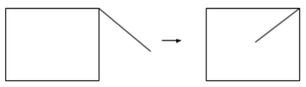
Graph on the right has longer edges when mapping to [25,675]^2 which helps obtaining ratio closer to desired ratios.”

Alternative solutions

I myself almost gave up early in this match by being unable to implement something relevant. Most probably that was because I was biased in my selection of the algorithm by the fact that I used the Spring-force based graph layouting method at work some years ago. The funny thing is that I managed to make it work after throwing it away for 4-5 times.
The core idea is the same as in the SA version of the solution: repeatedly unbend the edges. Take either an edge with lowest ratio, or the highest, and move both of its vertices as if there were a spring between them. In order for this method to converge, add a braking force that increases over time. Thus, in the beginning the the stiffness coefficient is much larger than in the end. This allows the system to oscillate for some time, and at some moments there appear quite a good states. These good states are recorded and the best of them is returned as a result.
I use a custom-written segment tree data structure for storing worst edges, and it turns out to be much faster than standard RB-tree/set.
mugurelionut uses essentially the same force-based idea, perhaps with a better tweak set.

chokudai’s solution

The provisional leader chokudai did not describe his solution for quite some time, so there was some mystery around his way of reaching 795, 760 points. Then he did publish a long-waited editorial, with Japanese version having wider explanation. He seems to use a variation of force-based approach, with some novel formulas to avoid spending time in bad states. Be sure to read the slides he shared.

Final notes

Make sure to check the Post your approach forum thread and read the other’s source code once it becomes available, because I tend to oversimplify these things. Then, take a good rest and see you in Round 2!