October 4, 2019 Image Classification with PyTorch
In the last post (Post) we saw how to create CNNs using PyTorch and also learned that CNNs are good at extracting important features from an image and converting them into vector representation for further processing. In short CNNs are very good at solving problems related to computer vision.
In this post we will be building an image classifier which will classify whether the image is of a ‘Cat’ or a ‘Dog’. Since there are only two classes for classification this is the perfect example of a binary image classification problem.
Steps for building an image classifier:
1. Data Loading and Preprocessing
“ The first step to training a neural network is to not touch any neural network code at all and instead begin by thoroughly inspecting your data – Andrej Karpathy, a recipe for neural network (blog)”
The first and foremost step while creating a classifier is to load your dataset. In PyTorch loading data is very easy. I trained my model on Google Collab so first we need to upload the image dataset to google drive.
#Importing Numpy Libraries
import numpy as np
import pandas as pd
from PIL import Image
import matplotlib.pyplot as plt
import torch
import torch.nn as nn
import torch.nn.functional as F
from torch.autograd import Variable
#import torch.utils.data as data
#from torch.utils.data import Dataset
from torchvision import transforms, datasets
from torch.utils.data import DataLoader, Dataset
import os
%matplotlib inline
#mounting google drive to access the dataset from drive folder
from google.colab import drive
drive.mount('/content/drive')

data_dir = "/content/drive/My Drive/Cat_Dog_Imageset"
train_dir = data_dir + '/training_set' # training_set contains training dataset
test_dir = data_dir + '/test_set'  #contains test dataset
We want our model to identify the images correctly irrespective of the size of an object in the image, i.e scale invariance, the angle of an object in an image, i.e rotation invariance, and alignment of an object in the image either left, right or center, i.e translation invariance. In summary we want the model to learn invariant representation of the image. A CNN has some built-in translation invariance which it achieves by applying Max Pooling layer. So in this step we will apply some transformation to our dataset such as random scaling, cropping, and image flipping. This will help the model to generalize, leading to better performance.
#Defining transformations for training and test data
#transforms.compose() will apply transformation to images
transformation = transforms.Compose([transforms.RandomHorizontalFlip(),
                                     transforms.RandomRotation(20),
                                     transforms.Resize(size=(224,224)),
                                     transforms.ToTensor(),
                                     transforms.Normalize((0.5, 0.5, 0.5), (0.5, 0.5, 0.5))
                                     ])
#Load the dataset with Image Folder
trainset = datasets.ImageFolder(train_dir, transform = transformation)
testset = datasets.ImageFolder(test_dir, transform = transformation)

#define data loaders
batch_size = 32
train_loader = DataLoader(trainset, batch_size=batch_size, shuffle=True,num_workers=2)
test_loader = DataLoader(testset, batch_size=batch_size,num_workers=1)
The data loader in PyTorch comes with numerous features such as data shuffling, loading the data in parallel using multiprocessing and ability to define batch size. These features help in consuming the data efficiently. PyTorch dataloader requires the following parameters: the dataset we want to load, batch size (number of training images in one training iteration), data shuffling, and how many workers we require for multi processing. Dataloader is the one which does the actual reading of the dataset.
ImageFolder is a generic data loader where the images are arranged in this way:
root/dog/1.jpg
root/dog/11.jpg

root/cat/xy23.jpg
root/cat/cat123.jpg
ImageFolder takes care of mapping image labels into classes. ImageFolder takes a reference from the folder name for classes. It expects folders and files to be constructed like above where each class is structured under its directory name (ex: Cat and Dog) for images. So image 1.jpg will belong to class cat and image xy23. Jpg belongs to class dog.
After the images are loaded and transformed we can visualize the images in the training set.
def imshow(img):
    img = img / 2 + 0.5  # unnormalize
    plt.imshow(np.transpose(img, (1, 2, 0)))  # convert from Tensor image
# obtain one batch of training images
data_iter = iter(train_loader)
images, lbls = data_iter.next()
images = images.numpy() # convert images to numpy for display
# plot the images in the batch, along with the corresponding labels
fig = plt.figure(figsize=(10, 4))
# display 20 images
for idx in np.arange(10):
    ax = fig.add_subplot(2, 10/2, idx+1, xticks=[], yticks=[])
    imshow(images[idx])
    label = lbls[idx]
    #ax.set_title(classes[label])
    ax.set_title(classes[lbls[idx]])

2. Creating a Model Using Convolutional Neural Network
Once the data is loaded then the next step is to build the network. Building CNN in PyTorch is relatively very simple. CNN in PyTorch is defined in the following way:
torch.nn.Conv2D(Depth_of_input_image, Depth_of_filter, size_of_filter, padding, strides)
#Creating CNN classifier
train_on_gpu = torch.cuda.is_available() #check if Cuda is available for training
#Initializing Parameters
class Net(nn.Module):
  def __init__(self):
    super(Net, self).__init__()
    # convolutional layer1
    self.conv1 = nn.Conv2d(3, 16, 5)
    # max pooling layer
    self.pool = nn.MaxPool2d(2, 2)
    # convolutional layer2
    self.conv2 = nn.Conv2d(16, 32, 5)
    self.dropout = nn.Dropout(0.2)
    # Fully connected layer1
    self.fc1 = nn.Linear(32*53*53, 256)
    # fully connected layer2
    self.fc2 = nn.Linear(256, 84)
   # fully connected layer3
    self.fc3 = nn.Linear(84, 2)
   # Applying softmax function
    self.softmax = nn.LogSoftmax(dim=1)
  # feed forward network
  def forward(self, x):
        # add sequence of convolutional and max pooling layers
        x = self.pool(F.relu(self.conv1(x)))
        x = self.pool(F.relu(self.conv2(x)))
        x = self.dropout(x)
        x = x.view(-1, 32 * 53 * 53)
        x = F.relu(self.fc1(x))
        x = self.dropout(F.relu(self.fc2(x)))
        x = self.softmax(self.fc3(x))
        return x


# create Model instance
model = Net()
print(model)

# move tensors to GPU if CUDA is available
if(train_on_gpu):
  model.cuda()
  print("CUDA available")
Output:
Net(
  (conv1): Conv2d(3, 16, kernel_size=(5, 5), stride=(1, 1))
  (pool): MaxPool2d(kernel_size=2, stride=2, padding=0, dilation=1, ceil_mode=False)
  (conv2): Conv2d(16, 32, kernel_size=(5, 5), stride=(1, 1))
  (dropout): Dropout(p=0.2, inplace=False)
  (fc1): Linear(in_features=89888, out_features=256, bias=True)
  (fc2): Linear(in_features=256, out_features=84, bias=True)
  (fc3): Linear(in_features=84, out_features=2, bias=True)
  (softmax): LogSoftmax()
)
CUDA available
Defining loss function and optimizer: loss function will measure the mistakes our model makes in the predicted output during the training time. It does so by calculating the difference between the true class label and predicted output label .
Here in this example we used Cross Entropy Loss since it is a multiclass classification problem. Once we find the errors, next we need to calculate how bad the model weights are – this is known as backpropagation. The next step is to optimize the weights in order to minimize the loss value; this is the role of the optimizer. The standard way of minimizing loss and maximizing best weight values is called Gradient Descent. In the example we used SGD (Stochastic Gradient Descent) as the optimizer.
import torch.optim as optim
# specify loss function
criterion = torch.nn.CrossEntropyLoss()
# specify optimizer
optimizer = torch.optim.SGD(model.parameters(), lr = 0.003, momentum= 0.9)
3. Training the Model
Training the model requires the following steps:
Initialize the epoch value, which is the number of iterations we want to run our model on the entire training dataset. Example: if we have a training dataset of 2000 images and the batch size is 500, then after 4 iterations, 1 epoch will complete.
i) Clear the previous gradients
ii) Forward Pass: computes the predicted output by passing the input to CNN model.
iii) Calculate Loss
iv) Backward Pass
v) Optimization
vi) Calculate average training loss
#Train Model
# number of epochs to train the model
n_epochs = 5 # you may increase this number to train a final model

#valid_loss_min = np.Inf # track change in validation loss

for epoch in range(1, n_epochs+1):

    # keep track of training and validation loss
    train_loss = 0.0
    #valid_loss = 0.0

    ###################
    # train the model #
    ###################
    model.train()
    for data, target in train_loader:
        # move tensors to GPU if CUDA is available
        if train_on_gpu:
            data, target = data.cuda(), target.cuda()
        # clear the gradients of all optimized variables
        optimizer.zero_grad()
        # forward pass: compute predicted outputs by passing inputs to the model
        output = model(data)
        # calculate the batch loss
        loss = criterion(output, target)
        # backward pass: compute gradient of the loss with respect to model parameters
        loss.backward()
        # perform a single optimization step (parameter update)
        optimizer.step()
        # update training loss
        train_loss += loss.item()*data.size(0)
    # calculate average losses
    train_loss = train_loss/len(train_loader.dataset)
    # print training/validation statistics
    print('Epoch: {} \tTraining Loss: {:.6f}'.format(
        epoch, train_loss))
Output:
Epoch: 1 	Training Loss: 0.681010
Epoch: 2 	Training Loss: 0.642268
Epoch: 3 	Training Loss: 0.613223
Epoch: 4 	Training Loss: 0.588775
Epoch: 5 	Training Loss: 0.572460
4. Evaluating Model Performance
Now is the time to test out the trained model on unseen data. For evaluating the model we will use model.eval(). By default the PyTorch network is in train() mode. But if the network has a dropout layer, then before you use the network to compute output values, you must explicitly set the network into eval() mode. The reason is that during training a dropout layer randomly sets some of its input to zero, which effectively erases them from the network, which makes the final trained network more robust and less prone to overfitting.
#Test Model
# track test loss
test_loss = 0.0
class_correct = list(0. for i in range(2))
class_total = list(0. for i in range(2))

model.eval()
i=1
# iterate over test data
len(test_loader)
for data, target in test_loader:
    i=i+1
    if len(target)!=batch_size:
        continue

    # move tensors to GPU if CUDA is available
    if train_on_gpu:
        data, target = data.cuda(), target.cuda()
    # forward pass: compute predicted outputs by passing inputs to the model
    output = model(data)
    # calculate the batch loss
    loss = criterion(output, target)
    # update test loss
    test_loss += loss.item()*data.size(0)
    # convert output probabilities to predicted class
    _, pred = torch.max(output, 1)
    # compare predictions to true label
    correct_tensor = pred.eq(target.data.view_as(pred))
    correct = np.squeeze(correct_tensor.numpy()) if not train_on_gpu else np.squeeze(correct_tensor.cpu().numpy())
    # calculate test accuracy for each object class
#     print(target)

    for i in range(batch_size):
        label = target.data[i]
        class_correct[label] += correct[i].item()
        class_total[label] += 1

# average test loss
test_loss = test_loss/len(test_loader.dataset)
print('Test Loss: {:.6f}\n'.format(test_loss))

for i in range(2):
    if class_total[i] > 0:
        print('Test Accuracy of %5s: %2d%% (%2d/%2d)' % (
            classes[i], 100 * class_correct[i] / class_total[i],
            np.sum(class_correct[i]), np.sum(class_total[i])))
    else:
        print('Test Accuracy of %5s: N/A (no training examples)' % (classes[i]))

print('\nTest Accuracy (Overall): %2d%% (%2d/%2d)' % (
    100. * np.sum(class_correct) / np.sum(class_total),
    np.sum(class_correct), np.sum(class_total)))
Output:
Test Loss: 0.497556

Test Accuracy of  cats: 86% (871/1011)
Test Accuracy of  dogs: 66% (668/1005)

Test Accuracy (Overall): 76% (1539/2016)
We got 76% accuracy on overall test data which is pretty good accuracy, since we used only 2 convolutional layers in our model. We tweak with a number of parameters such as number of convolutional layers, number of epochs, and adding more images to our dataset to increase the accuracy.
Visualizing Test Results:
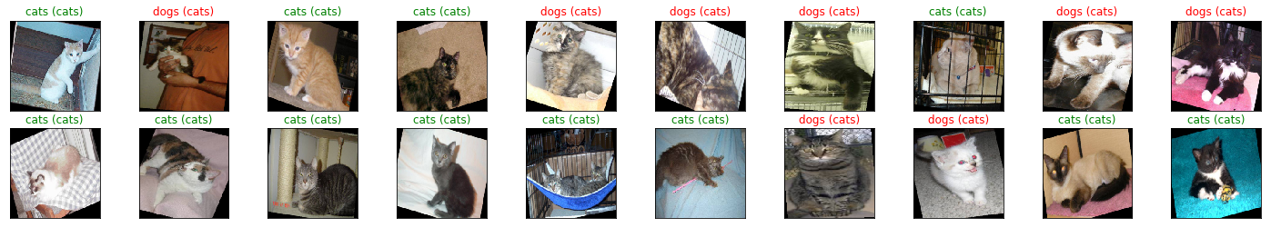
As you can see, our model predicted the wrong label a few times.
Conclusion: I hope you enjoyed reading the image classification example using PytTorch. You can check out the PyTorch data utilities documentation page which has other classes and functions to practice, it’s a valuable utility library.
rkhemka
Guest Blogger