By Zealint– Topcoder Member
The last part of the article introduces some well known applications of the minimum cost flow problem. Some of the applications are described according to [1].
The Assignment Problem
There are a number of agents and a number of tasks. Any agent can be assigned to perform any task, incurring some cost that may vary depending on the agent-task assignment. We have to get all tasks performed by assigning exactly one agent to each task in such a way that the total cost of the assignment is minimal with respect to all such assignments.
In other words, consider we have a square matrix with n rows and n columns. Each cell of the matrix contains a number. Let’s denote by cij the number which lays on the intersection of i-th row and j-th column of the matrix. The task is to choose a subset of the numbers from the matrix in such a way that each row and each column has exactly one number chosen and sum of the chosen numbers is as minimal as possible. For example, assume we had a matrix like this:
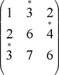
In this case, we would chose numbers 3, 4, and 3 with sum 10. In other words, we have to find an integral solution of the following linear programming problem:
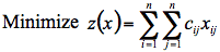
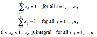
If binary variable xij = 1 we will choose the number from cell (i,j) of the given matrix. Constraints guarantee that each row and each column of the matrix will have only one number chosen. Evidently, the problem has a feasible solution (one can choose all diagonal numbers). To find the optimal solution of the problem we construct the bipartite transportation network as it is drawn in Figure 1. Each edge (i,j’) of the graph has unit capacity and cost cij. All supplies and demands are equal to 1 and -1 respectively. Implicitly, minimum cost flow solution corresponds to the optimal assignment and vise versa. Thanks to left-to-right directed edges the network contains no negative cycles and one is able to solve it with complexity of O(n3). Why? Hint: use the successive shortest path algorithm.
Figure 1. Full weighted bipartite network for the assignment
problem. Each edge has capacity 1 and cost according to the number in
the given matrix.
The assignment problem can also be represented as weight matching in a weighted bipartite graph. The problem allows some extensions:
Suppose that there is a different number of supply and demand nodes. The objective might be to find a maximum matching with a minimum weight.
Suppose that we have to choose not one but k numbers in each row and each column. We could easily solve this task if we considered supplies and demands to be equal to k and -k (instead of 1 and -1) respectively.
However, we should point out that, due to the specialty of the assignment problem, there are more effective algorithms to solve it. For instance, the Hungarian algorithm has complexity of O(n3), but it works much more quickly in practice.
Discrete Location Problems
Suppose we have n building sites and we have to build n new facilities on these sites. The new facilities interact with m existing facilities. The objective is to assign each new facility i to the available building site j in such a way that minimizes the total transportation cost between the new and existing facilities. One example is the location of hospitals, fire stations etc. in the city; in this case we can treat population concentrations as the existing facilities.
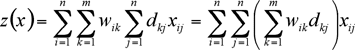
Let’s denote by dkj the distance between existing facility k and site j; and the total transportation cost per unit distance between the new facility i and the existing one k by wik. Let’s denote the assignment by binary variable xij. Given an assignment x we can get a corresponding transportation cost between the new facility i and the existing facility k:

The Transportation Problem
A minimum cost flow problem is well known to be a transportation problem in the statement of network. But there is a special case of transportation problem which is called the transportation problem in statement of matrix. We can obtain the optimization model for this case as follows.
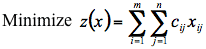
subject to
For example, suppose that we have a set of m warehouses and a set of n shops. Each warehouse i has nonnegative supply value bi while each shop j has nonnegative demand value dj. We are able to transfer goods from a warehouse i directly to a shop j by the cost cij per unit of flow.
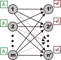
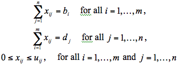
Figure 2. Formulating the transportation problem as a minimum cost flow problem. Each edge connecting a vertex i and a vertex j’ has capacity uij and cost cij.
There is an upper bound to the amount of flow between each warehouse i and each shop j denoted by uij. Minimizing total transportation cost is the object. Representing the flow from a warehouse i to a shop j by xij we obtain the model above. Evidently, the assignment problem is a special case of the transportation problem in the statement of matrix, which in turn is a special case of the minimum cost flow problem.
Optimal Loading of a Hopping Airplane
We took this application from [1]. A small commuter airline uses a plane with the capacity to carry at most p passengers on a “hopping flight.” The hopping flight visits the cities 1, 2, …, n, in a fixed sequence. The plane can pick up passengers at any node and drop them off at any other node.
Let bij denote the number of passengers available at node i who want to go to node j, and let fij denote the fare per passenger from node i to node j.
The airline would like to determine the number of passengers that the plane should carry between the various origins and destinations in order to maximize the total fare per trip while never exceeding the plane capacity.
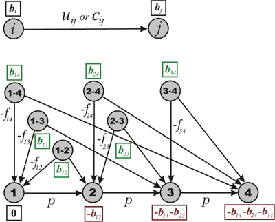
Figure 3. Formulating the hopping plane flight problem as a minimum cost flow problem.
Figure 3 shows a minimum cost flow formulation of this hopping plane flight problem. The network contains data for only those arcs with nonzero costs and with finite capacities: Any arc without an associated cost has a zero cost; any arc without an associated capacity has an infinite capacity.
Consider, for example, node 1. Three types of passengers are available at node 1, those whose destination is node 2, node 3, or node 4. We represent these three types of passengers by the nodes 1-2, 1-3, and 1-4 with supplies b12, b13, and b14. A passenger available at any such node, say 1-3, either boards the plane at its origin node by flowing though the arc (1-3,1) and thus incurring a cost of -f13 units, or never boards the plane which we represent by the flow through the arc (1-3,3).
We invite the reader to establish one-to-one correspondence between feasible passenger routings and feasible flows in the minimum cost flow formulation of the problem.
Dynamic Lot Sizing
Here’s another application that was first outlined in [1]. In the dynamic lot-size problem, we wish to meet prescribed demand dj for each of K periods j = 1, 2, …, K by either producing an amount aj in period j and/or by drawing upon the inventory Ij-1 carried from the previous period. Figure 4 shows the network for modeling this problem.
The network has K+1 vertexes: The j-th vertex, for j = 1, 2, …, K, represents the j-th planning period; node 0 represents the “source” of all production. The flow on the “production arc” (0,j) prescribes the production level aj in period j, and the flow on “inventory carrying arc” (j,j+1) prescribes the inventory level Ij to be carried from period j to period j+1.
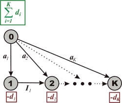
Figure 4. Network flow model of the dynamic lot-size problem.
The mass balance equation for each period j models the basic accounting equation: Incoming inventory plus production in that period must equal the period’s demand plus the final inventory at the end of the period. The mass balance equation for vertex 0 indicates that during the planning periods 1, 2, …, K, we must produce all of the demand (we are assuming zero beginning and zero final inventory over the planning horizon).
If we impose capacities on the production and inventory in each period and suppose that the costs are linear, the problem becomes a minimum cost flow model.
References
[1]Ravindra K. Ahuja, Thomas L. Magnanti, and James B. Orlin. Network Flows: Theory, Algorithms, and Applications.
[2]Thomas H. Cormen, Charles E. Leiserson, Ronald L. Rivest. Introduction to Algorithms.
[3]_efer_. Algorithm Tutorial: Maximum Flow.
[4]gladius. Algorithm Tutorial: Introduction to graphs and their data structures: Section 3.