July 22, 2021 Single Round Match 809 Editorials

OptimalGolf

When can we get a hole-in-one? Clearly, this is possible if and only if some of the clubs can hit distance D.

If we cannot get a hole-in-one, we will make at least two strokes.

Where can we land after the second stroke? Let M = max(clubHi) be the maximum distance we can hit in one stroke. Then we claim that after two strokes we can be completely anywhere within distance 2*M of the tee, and that we never need to use any other club, or use this club to hit any distance other than M.

For any point (x,0) with 0 <= x <= 2*M we can get from (0,0) to (x,0) in two strokes: the first to (x/2,y) and the second to (x,0), where y = sqrt(M*M – (x/2)*(x/2)). That is, we make two strokes of length exactly M each. For x=2*M we go directly, and the smaller x is, the more to the side we hit the first stroke.

For any other point withing 2*M from the tee we can reach it in exactly the same way, we just rotate ourselves by the appropriate angle before we start.

And we clearly cannot do anything else: whatever we do with clubs that have a shorter range, we will still be within the circle with radius 2*M of the tee.

Thus, if D <= 2*M and we cannot do a hole-in-one, we can get it in two strokes.

And now it should be obvious that for any D > 2*M the number of strokes we need is exactly S = ceiling(D/M), and we can always play the hole by making S strokes, each of length exactly M.

In other words, the answer is the smallest S such that S*M >= D.

On one hand, fewer strokes are clearly impossible – even if we hit distance M towards the hole each time, we would not get there in fewer than S strokes.

On the other hand, for S*M = D making S strokes is clearly optimal, and if S*M – D = x > 0, we can use the first two strokes to only traverse the distance 2*M-x instead of 2*M, and then each of the other S-2 strokes can go straight towards the goal.

Thus, the answer is either 1 if a hole-in-one is possible, or max(2,ceiling(D/M)) if it isn’t.

SimilarDNA

We are given two short strings and our task is to check whether their edit distance (Levenshtein distance) is at most 2. Levenshtein distance can be computed efficiently using dynamic programming, and if you know the algorithm, you could implement it and solve the task this way.

However, this was not necessary. The task is also solvable using brute force.

If we have a string of length N, we have 4(N+1) ways to make an insertion, N ways to make a deletion, and 4N ways to make a substitution (or only 3N if you only count substitutions where the letter actually changes.) For strings of length at most 51 this gives fewer than 500 different mutations. And thus there are fewer than 500^2 = 250,000 ways to make two consecutive mutations. We can simply generate all of them and check whether B is among them.

A sample implementation is shown below. We implement a function that does all possible single mutations and then use it twice. (Note a small trick out of laziness: when checking whether the edit distance is exactly two, we compare each string that has distance 1 from A and each string that has distance 1 from B. We can do this because mutations are symmetric. However, this trick does not improve the time complexity and it isn’t necessary. Instead, we could simply iterate over all x in left, for each of them call generateAll(x), and for each of those strings check whether it equals B.)

String[] generateAll(String A) {
    int N = A.length();
    String alphabet = "CGAT";
    String[] answer = new String[4*(N+1) + N + 4*N];
    int out = 0;

    // insertions
    for (int a=0; a<=N; ++a) for (int b=0; b<4; ++b)
      answer[out++] = A.substring(0,a) + alphabet.charAt(b) + A.substring(a);
    // deletions
    for (int a=0; a<N; ++a)
      answer[out++] = A.substring(0,a) + A.substring(a+1);

    // substitutions
    for (int a=0; a<N; ++a) for (int b=0; b<4; ++b)
      answer[out++] = A.substring(0,a) + alphabet.charAt(b) + A.substring(a+1);

    return answer;
}

public String areSimilar(String A, String B) {
    if (A.equals(B)) return "similar";
    String[] left = generateAll(A);
    for (String x : left) if (x.equals(B)) return "similar";
    String[] right = generateAll(B);
    for (String x : left) for (String y : right)
        if (x.equals(y)) return "similar";
    return "distinct";
}

LunchLine

There are many efficient solutions to this problem. A heavyweight solution is to use a strong enough data structure, but there are at least two much nicer and simpler solutions.

One option is to avoid implementing the operations one at a time. Instead, let’s just reconstruct the final queue.

Who is last? The person who was sent to the end most recently.

Who is in front of them? From everyone else, the person who was sent to the end most recently.

And so on. Eventually we’ll run out of kids that were sent to the end at least once. From that moment on, as we continue towards the front of the queue, we encounter all of the remaining kids in their original order.

This solution can easily be implemented in O(N+M) time: we just go through the sequence K backwards, and each time we encounter a new kid, we place it at the current beginning of the partially constructed final queue.

public long simulate(int N, int M, int A, int B, int C, int D, int E) {
    int[] K = new int[M];
    if (M > 0) K[0] = A;
    if (M > 1) K[1] = B;
    for (int i=2; i<M; ++i) K[i] = (int)( (1L*C*K[i-1] + 1L*D*K[i-2] + E) % N );
    int[] sequence = new int[N];
    boolean[] sent = new boolean[N];
    int where = N-1;
    for (int m=M-1; m>=0; --m) if (!sent[K[m]]) {
        sent[K[m]] = true;
        sequence[where--] = K[m];
    }
    for (int n=N-1; n>=0; --n) if (!sent[n]) sequence[where--] = n;
    long answer = 0;
    for (int n=0; n<N; ++n) answer += 1L*n*sequence[n];
    return answer;
}

Another solution is to stop being afraid to create gaps. In this solution we will remember the current position of each kid. In the beginning, kid i is in position i. The first time someone is sent to the end of the queue, we move them to the first position after the queue so far: position N. The second person sent to the end (even if it’s the same person as before) gets moved to position N+1. And so on. As we do this, we are maintaining the actual order of kids in the queue, the only caveat being the gaps between them. But there cannot be too many of those: the final kid will be placed at position N+M-1. In the end, we just traverse all N+M positions that may contain kids, skip the gaps and read the kids in the correct order.

A lazier implementation skips the last step and instead sorts records of the form (position[kid],kid) to get the kids’ final order. This introduces an extra logarithm for the sort but it is still plenty fast.

K = [A,B]
while len(K) < M: K.append( (C*K[-1] + D*K[-2] + E) % N )
while len(K) > M: K.pop()

position = list(range(N))
for m in range(M): position[K[m]] = N+m

kids = [ (position[n], n) for n in range(N) ]
kids.sort()

return sum( i*kids[i][1] for i in range(N) )

TruckUnion

This is clearly a variation of the Travelling Salesman Problem (TSP) and judging from N <= 18, we need to adapt the Bellman-Held-Karp exponential DP algorithm to work for our setting.

The number of cities T visited by each truck must be a divisor of N-1. Conveniently, this gives us only two options for the largest N=18 and five options for N=17, so those will be the worst cases. We will solve the problem separately for each T and pick the best of those solutions.

Once we fix T, we can proceed as follows. We will be sending the trucks one at a time: the first truck will visit the first T cities, the second one the second T cities, and so on. The states will be the moments when the current truck visits a city other than city 0. In our solution, we do the DP forwards: for each state we will compute the smallest total cost of reaching it. (The DP can also be done backwards, for each state we then compute the minimum cost of finishing the solution from that state. The two approaches are essentially equivalent and it’s just a matter of taste.)

More precisely, just like in the original algorithm, our states will be pairs (set of already visited cities, last visited city). As we do not care about city 0, we have at most 2^(N-1) * (N-1) states.

To initialize the starting states, for each state of the form ({x},x) the cost of reaching it is the cost of moving from city 0 to city x.

Now we can process all states in any order such that states reachable from any state S are only processed after S. If we use bitmasks to represent the sets of visited cities, the simple increasing order has this property. Once we have this property, each time we process a state, we know the optimal answer for that state, and we can now use it to find better solutions for some following states. More precisely, whenever we process a state (V,last), we consider all possibilities for which city we’ll visit next. This will move us from the current state to the state (V+{next},next).

And now that we have fixed T, this is the only place where our solution differs from the original algorithm. In our setting, what exactly is the cost of going from the state (V,last) to the state (V+{next},next)? This depends on the size of V. If the size of V is a multiple of T, the current truck ends its route and a new one begins, so the cost is the cost of going from last to 0 and then from 0 to next. Otherwise, the current truck continues its route and the cost we pay is the cost of going directly from last to next.

For a single T we have O(N2^(N-1)) states and for each of them O(N) work, so the total time complexity of this solution is O(D(N-1) * N^2 * 2^(N-1)), where D(x) is the number of divisors of x.

int N;
int[] popcount;
int[] Dout, Din;
int[][] D;

int solve(int t) {
    int Z = N-1;
    int[][] dp = new int[1<<Z][Z];
    for (int a=0; a<(1<<Z); ++a) for (int b=0; b<Z; ++b) dp[a][b] = 987654321;
    for (int z=0; z<Z; ++z) dp[1<<z][z] = Dout[z];
    for (int subset=1; subset<(1<<Z); ++subset) {
        for (int last=0; last<Z; ++last) {
            if ((subset & 1<<last) == 0) continue;
            for (int nxt=0; nxt<Z; ++nxt) {
                if ((subset & 1<<nxt) != 0) continue;
                int edge;
                if (popcount[subset] % t == 0) {
                    edge = Din[last] + Dout[nxt];
                } else {
                    edge = D[last][nxt];
                }
                dp[subset | 1<<nxt][nxt] = Math.min(
                    dp[subset | 1<<nxt][nxt], dp[subset][last]+edge );
            }
        }
    }
    int answer = 987654321;
    for (int last=0; last<Z; ++last)
        answer = Math.min(answer, dp[(1<<Z)-1][last] + Din[last] );
    return answer;
}

public int optimize(int _N, int[] C) {
    N = _N;

    Dout = new int[N];
    Din = new int[N];
    D = new int[N][N];
    for (int i=1; i<N; ++i) Dout[i-1] = C[0*N + i];
    for (int i=1; i<N; ++i) Din[i-1] = C[i*N + 0];
    for (int i=1; i<N; ++i) for (int j=1; j<N; ++j) D[i-1][j-1] = C[i*N+j];

    popcount = new int[1<<N];
    for (int i=1; i<(1<<N); ++i) {
        int x = i & (i-1);
        popcount[i] = popcount[x] + 1;
    }

    int answer = 987654321;
    for (int t=1; t<=N-1; ++t) if ((N-1) % t == 0)
        answer = Math.min( answer, solve(t) );
    return answer;
}

RectangleBreaking

Readers interested in the background behind this problem are encouraged to read the book Winning Ways for Your Mathematical Plays and/or the book On Numbers and Games. Both are written in a very accessible way and go much deeper than this editorial can aim to go.

In games like this one each position has a value that represents how many “extra” moves one of the players has in that position. In some partisan games these values can be non-integer (e.g., a position can give half a move advantage to one of the players), but luckily for us in this particular game all values will turn out to be integers.

If we knew how to compute these values, the analysis of a position would then be simple: if this value is zero, the game is of the “second” type, if the value is a positive or a negative integer, the player who has the guaranteed extra moves always wins. In this particular game positions of the “first” type cannot occur.

The values we are talking about are additive: if we have a sum of independent subgames (such as a collection of rectangles in our game), the value of the entire position is the sum of the values of the subgames. Showing this formally will require some background, but intuitively this should be pretty straightforward. For example, if we have two subgames such that in one of them one player has an extra move and in the other the other player has an extra move, these cancel each other out. The smallest non-trivial example is a position with a 2×1 rectangle and a 1×2 rectangle. One of them gives one move advantage to Hannah, the other gives one move to Victor, and together they create a “second”-type position: whoever is forced to start loses (if both play optimally).

TODO proof of the following claim: Let (r,c) be a rectangle. Its value can be computed as follows: let k be the biggest integer such that 2^k <= min(r,c). Then, the value of the rectangle is (r div 2^k) – (c div 2^k).

As a picture:

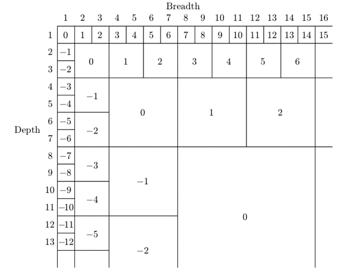
Once we know the value of each rectangle, we know the value of each position, and thus we can classify it.

If we have a position of value V != 0 and we add a rectangle 1 times (V+1) oriented in the other direction (i.e., one with value -V), we created a “second”-type position. Adding a bigger rectangle flips the balance towards the other player, adding a smaller rectangle (if possible) or a rectangle oriented in the same direction as the current value keeps it with the currently winning player.

And if we have a position of value V = 0, adding any rectangle creates a position where the player who got the extra moves wins.