June 28, 2019 Gradient Descent in Machine Learning

Before going into the details of Gradient Descent let’s first understand what exactly is a cost function and its relationship with the MachineLearning model.

In Supervised Learning a machine learning algorithm builds a model which will learn by examining multiple examples and then attempting to find out a function which minimizes loss. Since we are unaware of the true distribution of the data on which the algorithm will work so we instead measure the performance of the algorithm on known set of data i.e Training dataset. This process is known as Empirical Risk Minimization.
Loss is the penalty for a bad prediction, in simple terms it measures how well the algorithm is performing on the given dataset. Thus loss is a number which indicates how bad model prediction was on a single example. If the model prediction is 100% accurate then the loss will be zero else the loss will be greater. The function responsible for calculating the penalty is generally referred to as Cost Function.

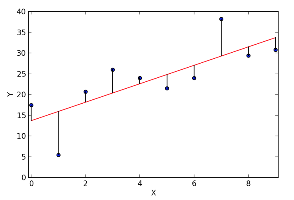
In the above image the farther the points is from the straight red line higher the error in predicted value w.r.t  ground truth value.

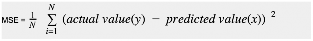
In this blogpost we will be discussing about the most popular Error/Loss function which is Mean Square Error.

Mean Squared Error(MSE) is calculated by taking the difference between the predicted output and the ground truth output , square the difference and then averaging it out across the whole dataset.

The primary goal of training a machine learning model is to find a set of weights and biases that have low loss on average across all examples i.e Minimising the Cost function.

This is  necessary because the lower error between the actual and predicted value signifies the model has learnt well i.e trained well on training dataset.

How to minimize cost function?

Gradient Descent in simple terms is an algorithm which minimizes a function. The general idea of Gradient Descent is to tweak parameters(weights and biases) iteratively in order to minimize a cost function. Suppose you are standing at the top of the mountain and you want to get down to the bottom of the valley as quickly as possible , the good strategy is to go downhill in the direction of steepest slope. This is exactly how gradient descent works, it measures the local gradient of the loss function with regards to parameter and it goes in the direction of negative gradient. Once the gradient is zero, you have reached the minimum.
Concretely , start by initializing with a random value and then improve it gradually taking one small step at a time , each step attempting to decrease the cost function(eg: MSE) , until algorithm converges to minimum.

with a random value and then improve it gradually taking one small step at a time , each step attempting to decrease the cost function(eg: MSE) , until algorithm converges to minimum.

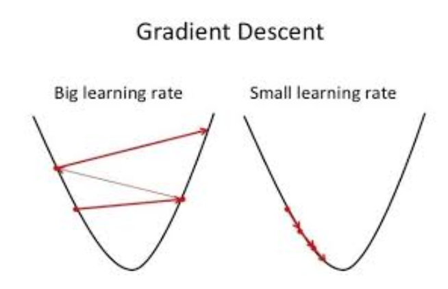
An important parameter in Gradient Descent is the size of step known as learning rate hyperparameter. If the learning rate is too small there will multiple iterations that the algorithm has to execute for converging which will take longer time. On the other hand, if the learning rate is too high , we might jump across the valley and end up on the other side , possibly even higher than before. This might make algorithm diverge with larger and larger values, failing to find a good solution.

Gradient Descent implementation steps

Step1: Initialize parameters (weight and bias) with random value or simply zero.Also initialize Learning rate.

Step2: Calculate Cost function (J)

Step3: Take Partial Derivatives of the cost function with respect to weights and biases(dW,db).

Step4: Update Parameter values as:

• Wnew =  W – learning rate * dW
• bnew = b – learning rate * db

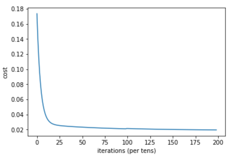
Step5: Repeat step2 to step 4 till n no of iterations. With each iteration the value of cost function will progressively decrease and eventually become flat value.

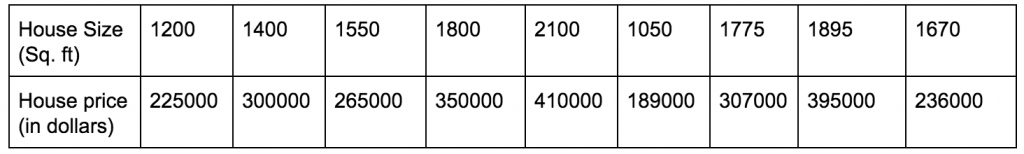
Let’s take an example of a dataset containing house sizes along with the house prices.

The example code needs Python 2.7 or higher version and requires following libraries:

1. Numpy for computation
2. Matplotlib for visualization

Python implementation of Gradient Descent Algorithm:

#importing necessary libraries
import numpy as np
import matplotlib.pyplot as plt
%matplotlib inline
# Normalized Data
X = [0,0.12,0.25,0.27,0.38,0.42,0.44,0.55,0.92,1.0]
Y = [0,0.15,0.54,0.51, 0.34,0.1,0.19,0.53,1.0,0.58]
Cost = []
#Initializing parameters
W = 0.45
B = 0.75
n_iter = 100 # no of iterations
#learning rate value set to 0.01
lr = 0.01
for i in range(1, 100):
  #Calculate Cost
  Y_pred = np.multiply(W, X) + b
  Loss_error = 0.5 * (Y_pred - Y)**2
  cost = np.sum(Loss_error)/10
  #Calculate dW and db
  db = np.sum((Y_pred - Y))
  dw = np.dot((Y_pred - Y), X)
  costs.append(cost)
  #Update parameters:
  W = W - lr*dw
  b = b - lr*db
  if i%10 == 0:
    print("Cost at", i,"iteration = ", cost)
#Repeat from Step2, implemented as a for loop with 100 iterations
#Plot the cost against no. of iterations
print("W = ", W,"& b = ",  b)
plt.plot(costs)
plt.ylabel('cost')
plt.xlabel('iterations (per tens)')

Output:

Cost at 10 iteration =  0.02098068740891688
Cost at 20 iteration =  0.020689041873919827
Cost at 30 iteration =  0.02044286360922784
Cost at 40 iteration =  0.02023200905713898
Cost at 50 iteration =  0.020051171528756562
Cost at 60 iteration =  0.01989605953945036
Cost at 70 iteration =  0.01976301202858763
Cost at 80 iteration =  0.019648890245194613
Cost at 90 iteration =  0.019551002036245543
W =  0.5725239059670542 & b =  0.148700522934184